The various deep learning works seen here are part of the Introduction to Deep Learning and Intermediate Deep Learning coursework at Carnegie Mellon University.

Airfoil Self-Noise Prediction Using a Multi-Layer Perceptron

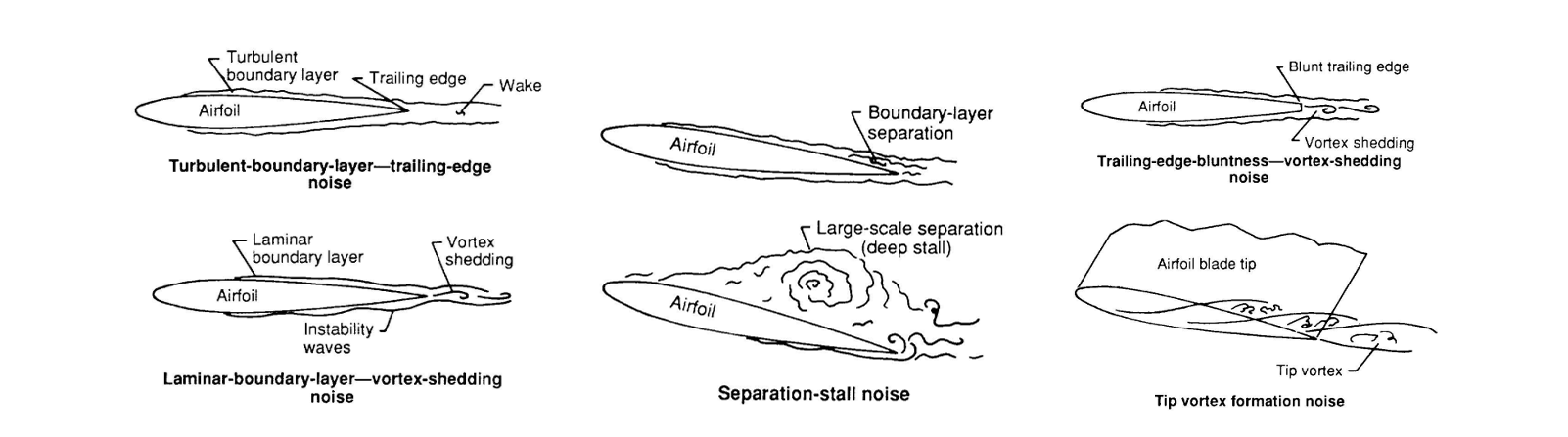
Airfoil noise factors

This work focused on developing a neural network to predict airfoil self-noise based on five input features: frequency, angle of attack, chord length, free-stream velocity, and suction side displacement thickness. The target output was the scaled sound pressure level in decibels. The task used a regression-based formulation, and the model was trained using PyTorch.

I implemented a custom Dataset class to load and batch the data (split into training, validation, and test sets), and defined a Multi-Layer Perceptron with configurable depth and width, along with a ReLU activation function. For evaluating the performance of the networks, and MSE loss was used

The network architecture, hyperparameters (learning rate, weight decay, batch size), and training loop were tuned across multiple configurations to evaluate their effect on model performance. Training was monitored using loss curves, and the best configuration, Combination 4, achieved a test loss of 11.913, indicating strong model generalization. I analyzed the impact of model depth, batch size, and learning rate on convergence rate and final error, and presented the results with accompanying plots.

Combination 1 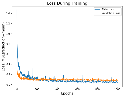hid_dim = [64, 32] num_epochs = 1000 lr = 0.01 weight_decay = 1e-5 batch_size = 32 Train Loss: 0.4474 Validation Loss: 0.7819 TOTAL EVALUATION LOSS: 16.13764 Increasing the number of neurons improved the model's performance on the test dataset by reducing the test loss. However, model 1 didnt generalize well enough as evidenced by the difference in training and validation losses.

Combination 2 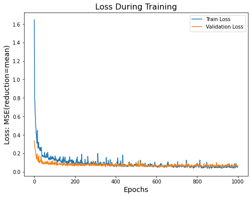hid_dim = [32, 64] num_epochs = 1000 lr = 0.01 weight_decay = 1e-5 batch_size = 32 Train Loss: 0.4739 Validation Loss: 0.5971 TOTAL EVALUATION LOSS: 14.82711 The validation and training are very close, indicating a good amount of generalization. The plots are still jittery, likely due to a high learning rate.

Combination 3 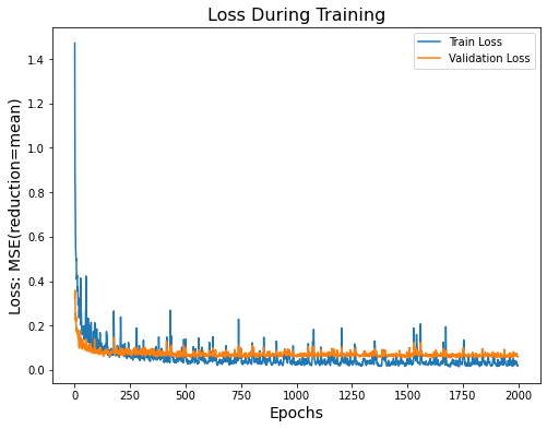hid_dim = [32, 64, 32] num_epochs = 2000 lr = 0.01 weight_decay = 1e-5 batch_size = 32 Train Loss: 0.2237 Validation Loss: 0.5934 TOTAL EVALUATION LOSS: 12.83629 The loss plots appear jittery, likely due to the high learning rate. However, adding an extra layer and running for more epochs appears to have improved the model's performance on the test data. The validation loss is higher than the training loss, indicating a minor degree of overfitting.

Combination 4 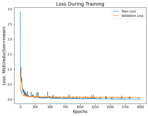hid_dim = [64, 128, 256, 256, 128, 64] num_epochs = 2500 lr = 0.0005 weight_decay = 1e-6 batch_size = 128 Train Loss: 0.0233 Validation Loss: 0.1845 TOTAL EVALUATION LOSS: 11.91328 A wider and deeper neural network, along with a learning rate of 0.0005 and a batch size of 128, gave the lowest error on the test data. The complexity of the network and the larger batch size had the most impact in lowering the test error. The test loss curve's spikes indicate that the learning rate may be too high initially.

References

Thomas F. Brooks, D. Stuart Pope, and Michael A. Marcolini. Airfoil self-noise and prediction. NTRS Author Affiliations: PRC Kentron, Inc., Hampton, NASA Langley Research Center NTRS Report/Patent Number: L16528 NTRS Document ID: 19890016302 NTRS Research Center: Legacy CDMS (CDMS). July 1989. Url: https://ntrs.nasa.gov/citations/19890016302 (visited on 01/24/2023).

RobertoLopez.Airfoil Self-Noise Data Set. Mar. 2014. URL: https://archive.ics.uci.edu/ml/datasets/airfoil+self-noise.

CIFAR-10 Image Classification Using a Convolutional Neural Network

In this exercise, I implemented a Convolutional Neural Network (CNN) to perform image classification on the CIFAR-10 dataset, which consists of 60,000 32×32 color images across 10 object categories. The goal was to train a model that generalizes well to unseen data while avoiding overfitting, using PyTorch as the primary framework.

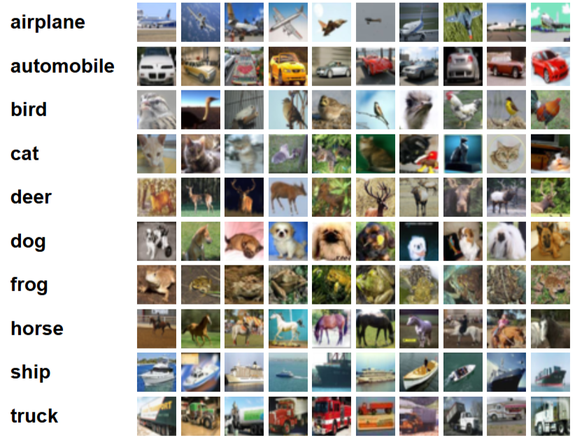
CIFAR-10 Dataset

Network Architecture

The training pipeline included dataset normalization, data augmentation with random 45 degree rotation, random crop and random vertical flip, and network regularization using dropout. I defined a ResNet inspired CNN architecture consisting of multiple convolutional layers with ReLU activation and max-pooling, followed by fully connected layers for classification. Cross-entropy loss was used with the Adam optimizer.

Training

During training, I monitored both training and validation loss and accuracy, and tuned the model to maximize test performance.

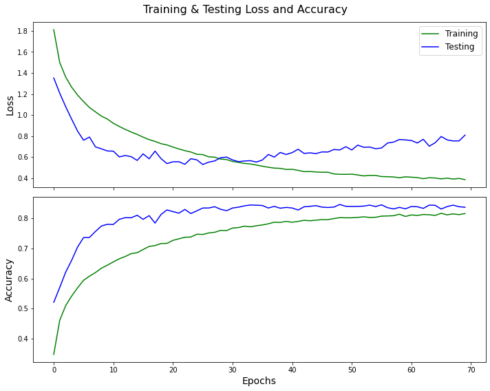
Loss and Accuracy over training

The final model was trained for 50 epochs and achieved a test accuracy of 83.63%, demonstrating strong classification performance across multiple classes. Several incremental improvements were made during the development process. Initially, the batch size was increased from 4 to 128, random rotation was introduced up to 45 degrees, and the base model was expanded with additional layers and ReLU activations. Switching to the Adam optimizer with a learning rate of 0.001 and training for 30 epochs yielded ~66% accuracy, which improved to ~72% after 50 epochs. Adding three more convolutional layers and an additional linear layer resulted in the model stalling at ~10% accuracy, indicating poor training behavior. This was addressed by removing the last three convolutional and max-pooling layers and introducing dropout with a 25% probability, which improved accuracy to ~79%. Further augmentation with random cropping and vertical flipping brought the performance to ~80%. Finally, a ResNet-based architecture was implemented, with one residual and two convolutional layers removed to reduce the number of trainable parameters from ~15 million to ~9 million, reducing underfitting.

References

CIFAR 10 Dataset: www.cs.toronto.edu/~kriz/cifar.html

Graph Neural Network for Molecular Solubility Prediction

This undertaking explored the use of Graph Neural Networks (GNNs) for predicting aqueous solubility from molecular structure, using PyTorch Geometric. Each molecule was represented as a graph with atoms as nodes and bonds as edges. Node and edge features were precomputed, and the task was framed as a regression problem to predict log solubility.

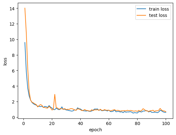
I implemented a GCN-based model using the GCNConv layer from torch_geometric.nn, and trained it using mean squared error (MSE) loss. The dataset was preprocessed, and the training loop was augmented with early stopping and model checkpointing to prevent overfitting. The model was configured with 8 graph convolutional layers, each using 128 channels, followed by a single linear layer that maps the 128-dimensional output to the final prediction. Batch normalization was applied after convolutional layers 1, 2, 3, 5, and 6, with the selection based on trial and error. The training objective used mean squared error loss (nn.MSELoss) appropriate for the regression task. Optimization was performed using Adam with a learning rate of 0.0001 and weight decay of 1e-5. The model was trained for 100 epochs, which provided the best balance between underfitting and overfitting. The model met performance expectations by achieving a sum of mean square errors between the model prediction and the label of 167.

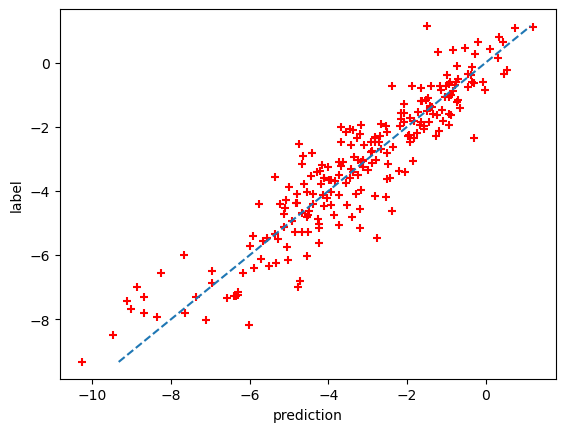Left: Loss over training, Right: Prediction vs Label.

References

Kipf, Thomas N., and Max Welling. “Semi-supervised classification with graph convolutional networks.” arXiv preprint arXiv:1609.02907 (2016).

LSTM Modeling of Transient Hagen–Poiseuille Flow

To learn the evolution of the axial velocity field from initial flow conditions, I trained an LSTM model to predict the transient velocity profile of incompressible laminar flow through a pipe, governed by the simplified Navier–Stokes equations for Hagen–Poiseuille flow. I implemented a multi-layer LSTM using PyTorch’s nn.LSTMCell, enabling step-wise control over hidden states. The model was trained on a dataset consisting of velocity measurements at 17 spatial points over 20 time steps, where each input sequence began with physical flow parameters (diameter, pressure gradient, viscosity, density) followed by 19 steps of observed velocity. During testing, only the initial condition was provided to autoregressively predict the entire 20-step sequence.

Training

Training was performed using MSE loss and the Adam optimizer, with tuned hyperparameters to minimize L1 and L2 errors. The model was evaluated by comparing predicted flow profiles to the true time evolution across the pipe radius. The model was initially trained using three LSMCell layers with a batch size of 128 and dropout set to 0.1; however, this configuration yielded poor predictions, with L1 and L2 losses in the ranges of 1e-5 and 1e-3, respectively. After resolving shape and datatype mismatches, I reduced the model to two LSMCell layers, adjusted the batch size to 64, and increased the dropout rate to 0.15, which slightly improved the results but still produced unsatisfactory predictions. The final breakthrough occurred after correcting a timestep loop error in the forward and test methods, which resolved the prediction issue and yielded acceptable L1 and L2 losses. The final training setup consisted of 20 epochs, a learning rate of 0.001, a dropout rate of 0.15, and a batch size of 64.

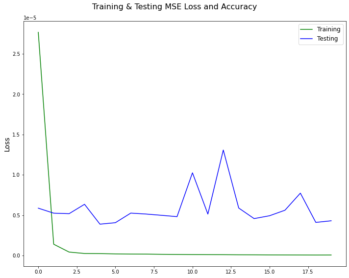
Loss over training

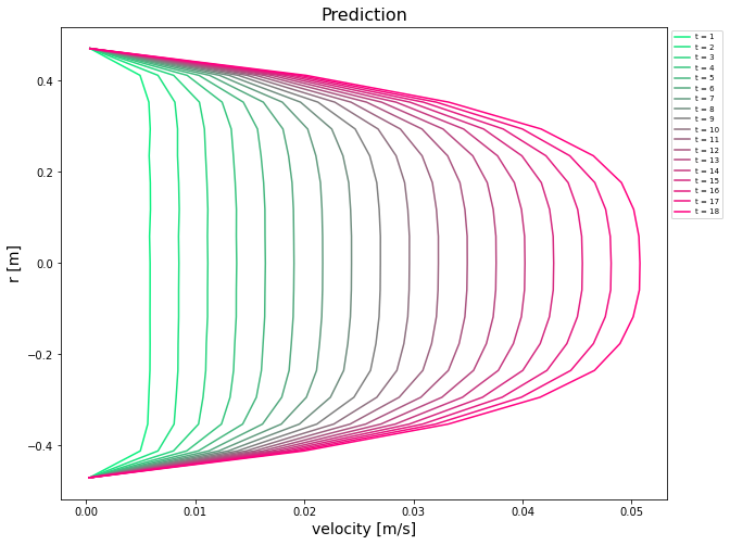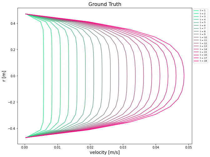Left: Prediction, Right: Truth.

The final model achieved a total L1 error of 4580.517 and L2 error of 14.075, meeting satisfactory performance. This exercise demonstrates how sequence learning methods like LSTM can effectively capture temporal dynamics in physical systems governed by PDEs, and serve as surrogates for numerical solvers.

References

The course assignment guide.

Nina Prakash for providing her code for generating Hagen-Poiseuille flow data.

Airfoil Shape Generation Using Variational Autoencoders and Generative Adversarial Networks

In this assignment, I generatively modeled airfoil geometries using Variational Autoencoders (VAEs) and Generative Adversarial Networks (GANs). The input dataset consisted of 1,600 airfoil shapes from the UIUC Airfoil Database, which were preprocessed by interpolating to a shared x-coordinate grid and scaling the y-coordinates to the range [−1, 1]. The generative models were trained to learn the underlying distribution of airfoil shapes using only the y-coordinates as input.

VAE model

The VAE architecture employed a 3-layer encoder (256–512–512 units) and a 2-layer decoder (512–512 units), each with ReLU activations and a final Tanh activation in the decoder. The model was trained for 30 epochs using an MSE loss term, weighted equally, with a small KL divergence regularization term (weight = 0.0001). Adam optimizer was used with a learning rate of 0.001. Tuning included expanding layer widths and deepening the encoder and decoder to improve expressiveness. The resulting generated airfoils were consistent and realistic, although the diversity of shapes was somewhat limited.

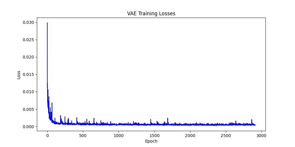
Loss over training

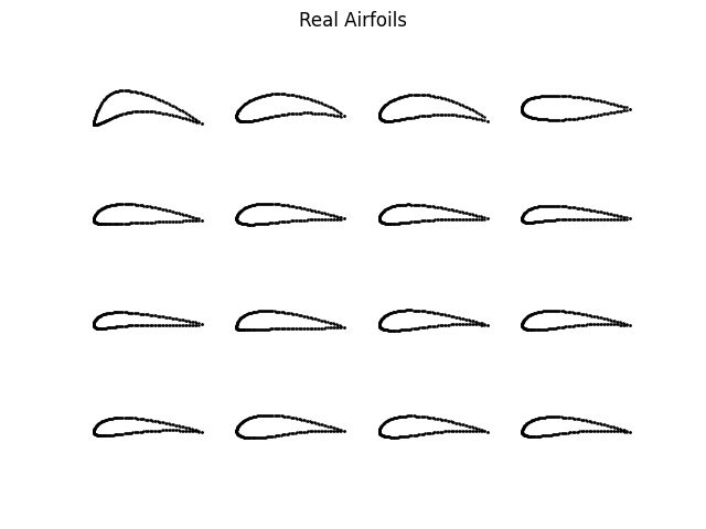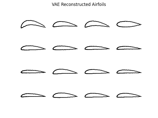Left: Real Airfoils, Right: VAE Reconstructed Airfoils

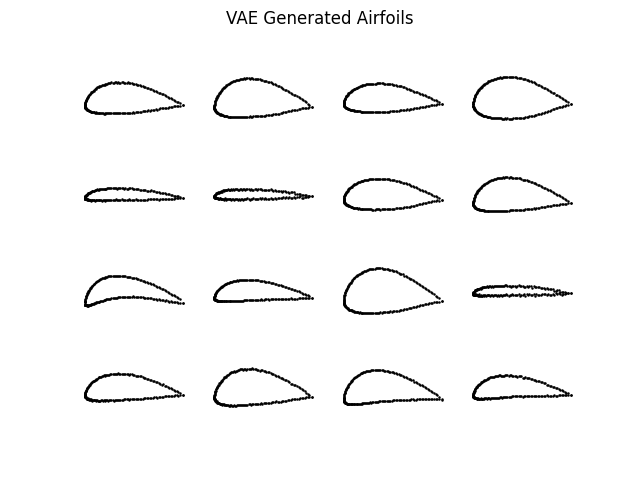
VAE Generated Airfoils

GAN model

The GAN was trained with a 4-layer generator (128–256–512–1024 units) and a 2-layer discriminator (512–256), utilizing LeakyReLU activations throughout, with a Sigmoid activation at the output of the discriminator and a Tanh activation in the generator. Batch normalization was applied after generator layers 1, 2, and 4 to stabilize the training process. The model was trained for 60 epochs using the Adam optimizer with a learning rate of 0.0005 for both the generator and discriminator.

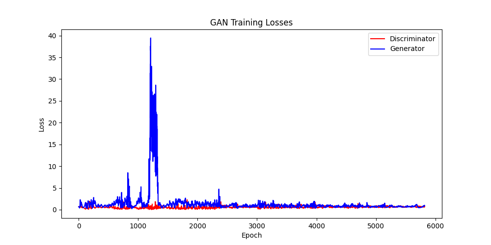
Loss over training

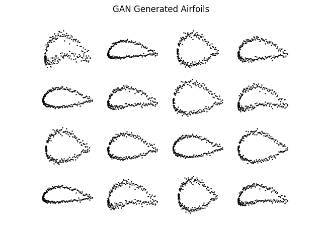
VAE Generated Airfoils

Comparison

The VAE-generated shapes were smoother and more interpretable, indicating strong reconstruction accuracy and clear latent space structure. Meanwhile, the GAN produced more visually diverse but fuzzier outputs, suggesting better sampling diversity at the cost of precision. This highlights a fundamental tradeoff between clarity and exploration in generative design models.

References

The course assignment guide.

Face Image Generation Using GAN on CelebA Dataset

Using Generative Adversarial Networks (GANs), I synthesized realistic face images by training my model on the CelebA dataset, which consists of 49,736 RGB face images. The images were each resized to 128×128×3 to be training input to the model.

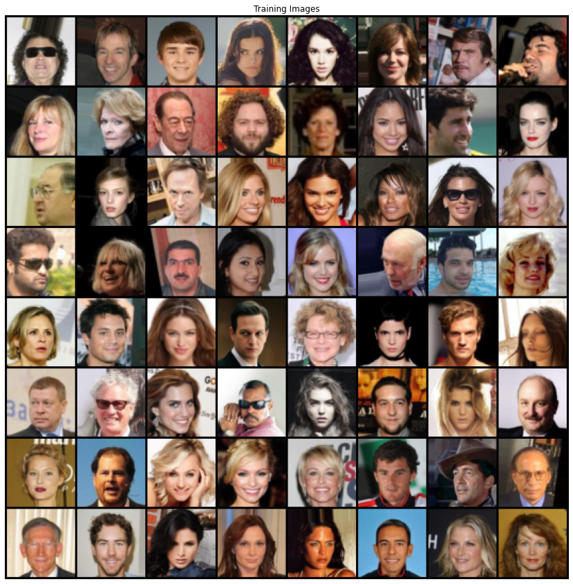
CelebA Dataset

The GAN architecture consisted of a generator network that learned to map Gaussian noise vectors to synthetic images, and a discriminator that learned to classify real versus fake images using binary cross-entropy loss. Both networks were trained iteratively using the standard adversarial training loop. PyTorch was used for implementation and training on Google Colab with GPU acceleration.

Generator

The generator consisted of a 5-layer transposed convolutional network:

• Input: 100-dimensional Gaussian noise vector
• ConvTranspose layers with increasing spatial resolution: 4×4 -> 8×8 -> 16×16 -> 32×32 -> 64×64 -> 128×128
• Channel progression: 512 -> 256 -> 128 -> 64 -> 3
• Batch normalization after each hidden layer
• Activations: ReLU for all hidden layers, Tanh for the output layer to match normalized image range

Discriminator

The discriminator was a mirrored 5-layer convolutional network:

• Input: 128×128×3 RGB image
• Convolutional layers with downsampling: 128×128 -> 64×64 -> 32×32 -> 16×16 -> 8×8 -> 4×4
• Channel progression: 3 -> 64 -> 128 -> 256 -> 512
• Batch normalization after all but the first layer
• Activations: LeakyReLU throughout with a final Sigmoid for binary output

Training

Training utilized binary cross-entropy loss (nn.BCELoss()) for both networks, along with the Adam optimizer with β1 = 0.5 and a learning rate of 0.0002. The networks were trained for 200 epochs with a batch size of 128. Training was stabilized using label smoothing (real labels as 0.9) and alternating update steps between generator and discriminator.

Loss values were tracked during training and plotted over iterations to monitor convergence. Generator loss generally decreased while discriminator loss oscillated, reflecting the adversarial dynamic.

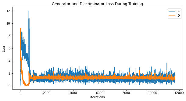
Loss over training

The final model generated visually plausible faces with correct facial proportions, realistic shading, and skin tone variation. Generated faces displayed learned symmetries and structure but occasionally exhibited artifacts such as blurry features or asymmetries, especially in early epochs.

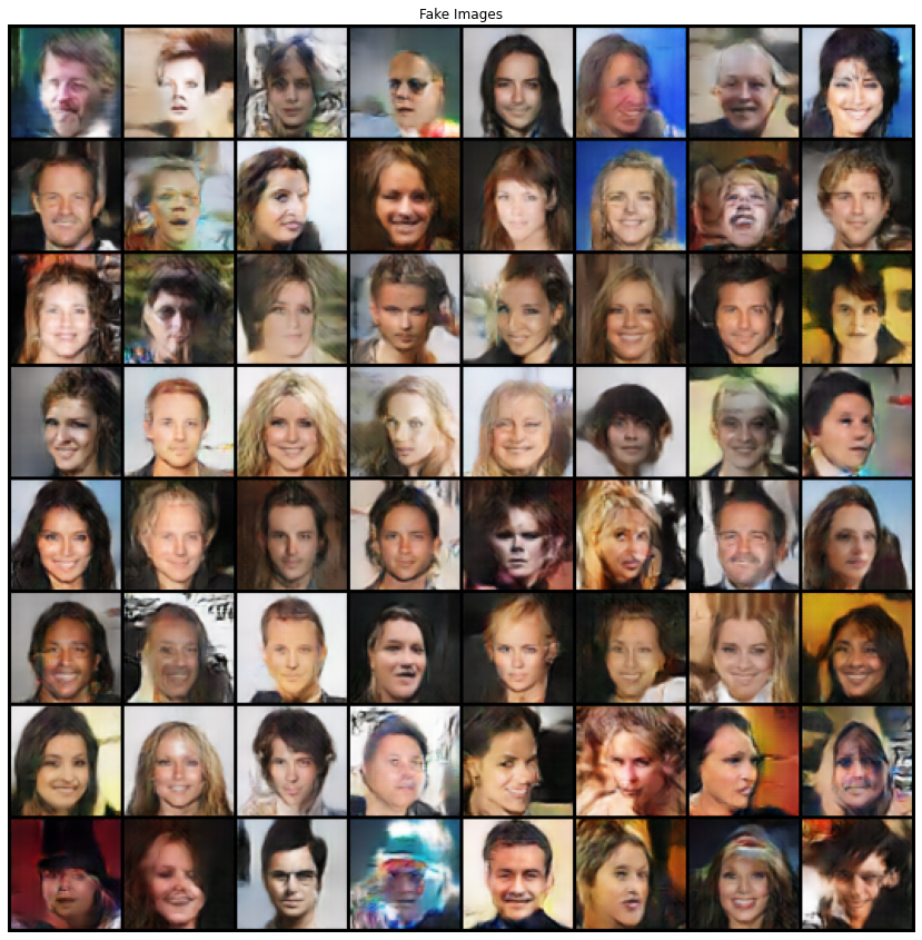
GAN generated faces

References

The course assignment guide.

Image Generation Using Denoising Diffusion Probabilistic Models

I implemented a Denoising Diffusion Probabilistic Model (DDPM) to generate synthetic images of the digits “1” and “5” from the MNIST dataset. DDPMs operate by progressively adding Gaussian noise to images during a forward diffusion process and then learning to reverse this process to generate realistic data. A UNet-based architecture was trained to model this reverse trajectory by predicting the noise component at each step.

The UNet consisted of four downsampling blocks, followed by symmetrical upsampling blocks, with concatenated skip connections at each level. Each block used Conv2D layers, GroupNorm, SiLU activations, and temporal embedding additions. Timestep embeddings were generated using sinusoidal encodings followed by MLP projection.

The model was trained for 100 epochs using a batch size of 128 and an initial learning rate of 1e-3. Training was performed on GPU with PyTorch, and the loss consistently decreased as the model learned to better denoise samples across all diffusion steps. After training, the model was used to generate 36 diverse samples of the digits “1” and “5” by progressively denoising Gaussian noise. The results showed well-formed structures that captured the statistical properties of the training data. To qualitatively understand the generation process, denoising trajectories were plotted for individual samples. These showed smooth transitions from noise to structured digits, highlighting the learned stochastic refinement behavior across steps.

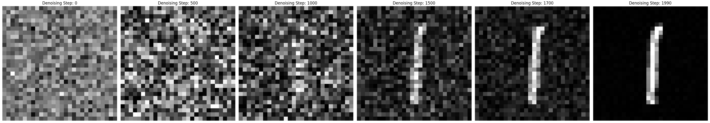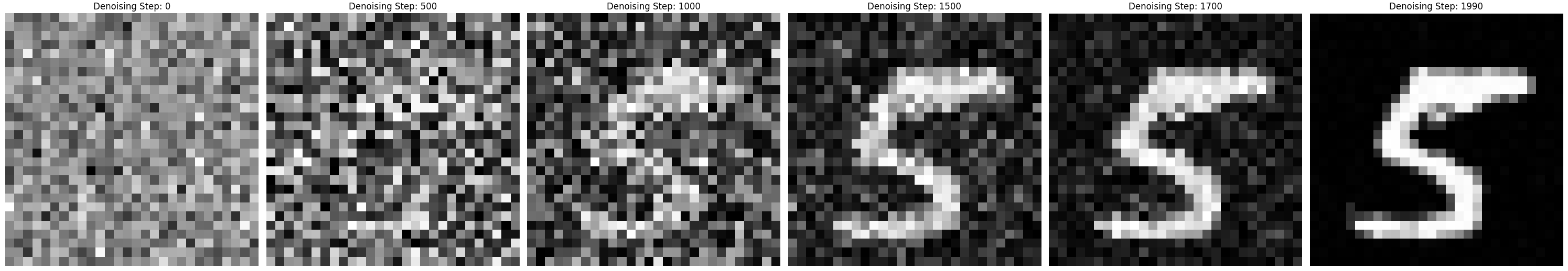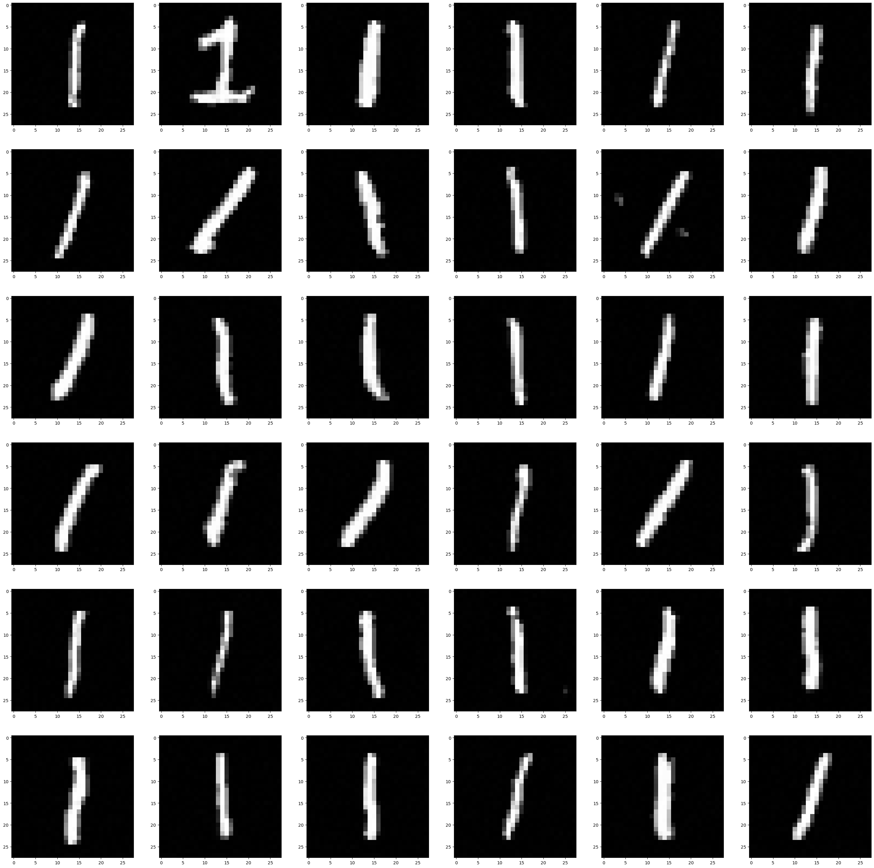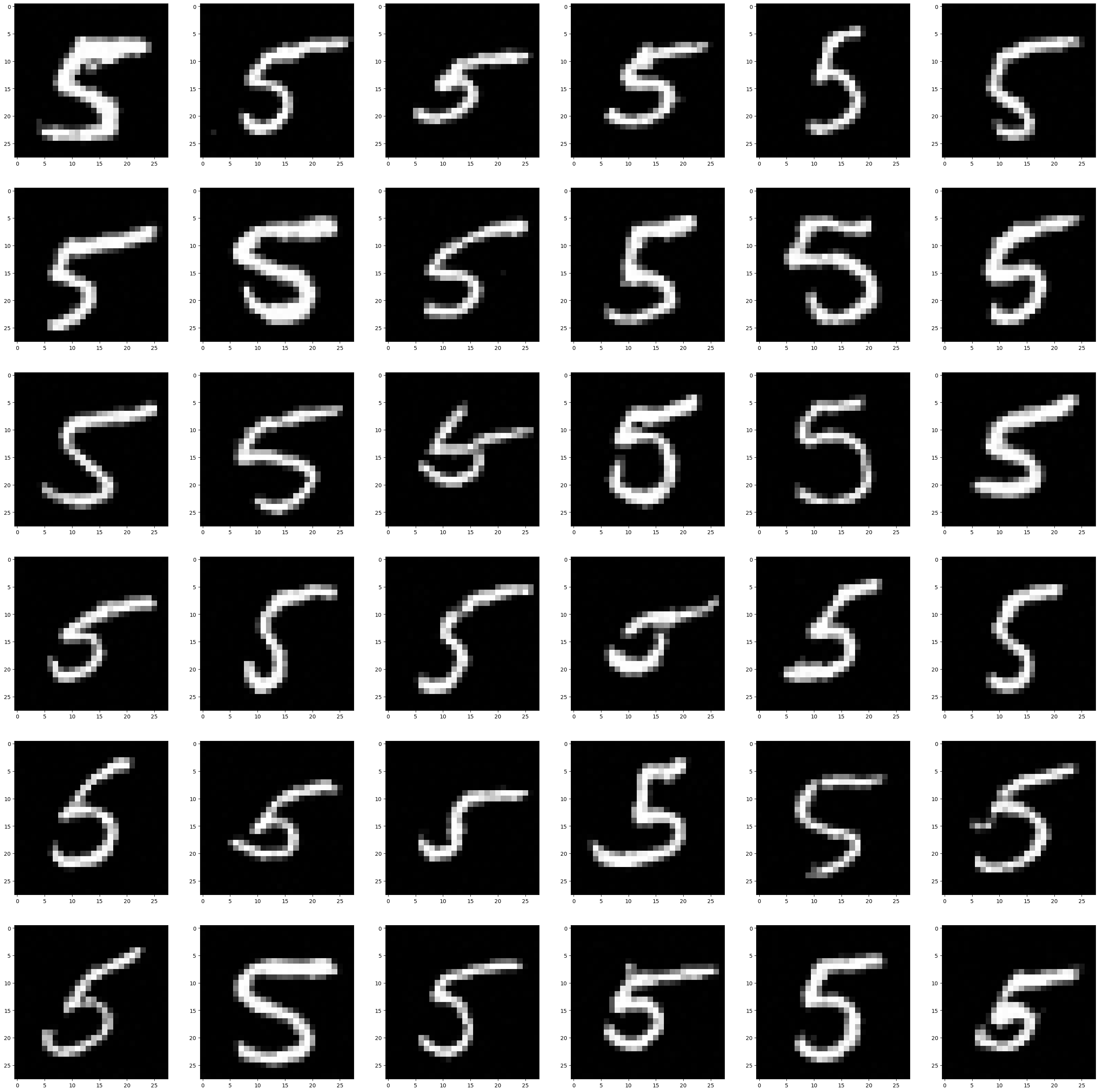Visualization of denoising and the final diffusion denerated samples

References Ho, Jonathan, Ajay Jain, and Pieter Abbeel. “Denoising diffusion probabilistic models.” Advances in neural information processing systems 33 (2020): 6840-6851.