
Control Stabilization for Bi-Quadcopter Payload Delivery System
Introduction
In recent years, drones have emerged as versatile tools, significantly impacting sectors like agriculture, surveillance, and delivery. While their applications are expansive, a primary limitation hindering broader usage is the restricted payload capacity. Traditional single-drone designs are often inadequate for tasks requiring substantial load carriage. This paper examines an innovative approach to address this challenge: the Bi-Quadcopter Payload Delivery System. This system features a novel integration of two drones connected by a specially designed truss structure. The primary objective of this design is to enhance the payload capacity beyond the limitations of conventional single-drone systems. By distributing the load between two interconnected drones, the system aims to achieve greater stability and efficiency in payload delivery. The motivation for this project stems from the growing demand for drones capable of transporting larger payloads across various industries. This demand is particularly evident in sectors where drones are increasingly preferred for their ability to navigate challenging terrains, enhance efficiency, and reduce human risk in operations. However, the limited payload capacity of current drone technology often necessitates compromises in operational scope and efficiency.
Methodology
The first step in enabling the bi-quadcopter flight was iteratively designing a robust truss structure that is light weight. Polylactic Acid (PLA) was used to maintain the lightweight nature. The truss strategically positioned the payload at the center, balancing it between the two drones. This positioning, coupled with the symmetry of the CrazyFlie drones’ motors and arms, resulted in a exploitable symmetry in controller design logic.
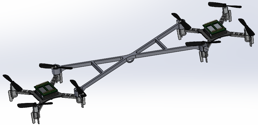
SolidWorks Assembly of the Dual-Drone System. Note the cross shape of the truss allowing for an unobstructed view for the Flowdecks on the underside
The bi-quadcopter setup’s system modelling involved develop a state-space dynamics model that accurately represented the behavior and responses of the interconnected drones. This model is vital for predicting the system’s performance under various load conditions and flight scenarios. The existing Crazyflie cascaded Proportional-Integral-Derivative (PID) controller was redesigned and tuned to match the new dual drone dynamics. This controller modification was essential for achieving precise and stable flight control, considering the additional complexity about the roll and yaw flight operation due to the design. In addition, a setpoint change was made for yaw operations that significantly improved performance
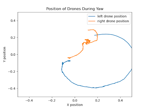 | 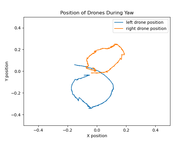 |
x and y coordinates of both drones during yaw. Left: With default setpoint, Right: With modified setpoint
Simulink was used to assess the response of the new controller on the hardware, providing a virtual testing ground for our controller tuning process. For payload pickup, rigid donut-shaped magnets were used along with a payload comprised of a heap of magnetic paper clips. Each magnet and paperclip weighed approximately 3g and 0.5g respectively. to further stabilize the flight operations after the payload pickup process, an adaptive controller was implemented. This controller dynamically adjusted the PID settings based on the weight of the payload, ensuring consistent performance across a range of payloads.
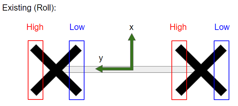 | 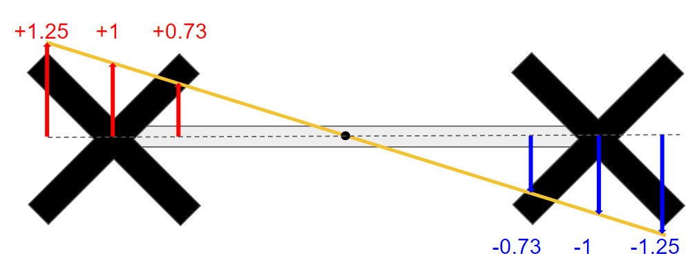 |
Left: Default power distribution in roll direction, Right: Modified power distribution in roll direction
Results
Initially, the drone underwent calibration without added mass, aiming to minimize steady-state roll error before payload pick-up operations. This pre-tuning phase revealed a mean error of about 8.5%, coupled with significant oscillations and instability, as detailed in the following figure. The drone executed left and right translations over 2 meters at 0.3 meters/second. Notably, introducing a delay between directional changes enhanced stability.
Average.png) | Average.png) |
No mass roll PID tuning. Left: Default PID values, Right: Tuned PID values
Following this, the drone was calibrated with an added mass of approximately 8 grams to further reduce steady-state roll error during payload transport. Pre-tuning, shown in below, indicated a mean error around 7.4% with similar instability to the initial tests. The control commands mirrored those of the no-mass phase, involving lateral movements across 2 meters at 0.3 meters/second. Tuning successfully reduced the mean error to 5.8% and enhanced stability.
Average.png) | Average.png) |
With mass roll PID tuning. Left: Default PID values, Right:Tuned PID values
Overall, the results demonstrated the practical viability of the Bi-Quadcopter Payload Delivery System. The system not only achieved its primary goal of increased payload capacity but also maintained the essential attributes of stability and control, paving the way for its potential application in various industrial and commercial sectors.
| Single Drone | Bi-Quadcopter | % change | |
|---|---|---|---|
| Payload Capacity [g] | 7 | 10 | 43 % increase |
| Lateral Translation Mean Error [%] | 7.8 | 5.8 | 26 % decrease |
Conclusion
The project demonstrated that the dual drone system, after stabilization, supports a higher payload than a single drone. Further enhancements were observed with the application of the adaptive controller. This advanced control allowed the drone to efficiently execute the load pickup, compare baseline and measured PWM, and appropriately scale PID values. With the tuned PID gains, the drone successfully performed the left-right lateral translation test for roll flight operation, affirming the effectiveness of the overall control system.
To conclude, the integration of two CrazyFlie drones, connected via a rigid 3D printed truss and equipped with a magnet-based payload delivery mechanism, marks a significant advancement. Our dynamics model, leveraging state space representation and onboard Cascaded PID controllers, ensured precise control. Addressing initial stability issues through firmware adjustments and the adaptive controller adjusting for payload variations, resulted in a notably stable and smooth operation of the bi-quadcopter system.
Team
Our final presentation is available to view here
Our final report is available to view here
The full playlist of videos of our testing and final demo result can be found on YouTube
The team consisted of Peter Blumenstein, who worked on simulation tasks; Srikumar Brundavanam, who was involved in firmware development and swarm flight implementation; Shang Shi on firmware development and hardware testing and tuning; Ben Spin, on truss design and dynamics modeling; and myself working on dynamics modeling, controller design, and hardware testing & tuning.
Acknowledgements
We would like to express our sincere gratitude to Dr. Mark Bedillion, whose expertise, understanding, and patience, added considerably to our experience and understanding of control systems and their implementation. We would also like to thank Dr. Aaron Johnson for his assistance in developing the dynamics model of our project. Additionally, we are indebted to Khai Nguyen, the teaching assistant for 24-774 Special Topics: Advanced Control Systems Integration for Fall 2023, for his invaluable assistance throughout this project. H
References
J.-P. Aurambout, K. Gkoumas, and B. Ciuffo, “Last mile delivery by drones: An estimation of viable market potential and access to citizens across European cities,” European Transport Research Review, vol. 11, no. 1, 2019. doi:10.1186/s12544-019-0368-2
J. E. Scott and C. H. Scott, “Models for drone delivery of medications and other healthcare items,” Unmanned Aerial Vehicles, pp. 376–392, 2019. doi:10.4018/978-1-5225-8365-3.ch016
Mohsan, S.A.H., Othman, N.Q.H., Li, Y. et al. Unmanned aerial vehicles (UAVs): practical aspects, applications, open challenges, security issues, and future trends. Intel Serv Robotics 16, 109–137 (2023). https://doi.org/10.1007/s11370-022-00452-4
D. G. Morín, J. Araujo, S. Tayamon and L. A. A. Andersson, “Autonomous Cooperative Flight of Rigidly Attached Quadcopters,” 2019 International Conference on Robotics and Automation (ICRA), Montreal, QC, Canada, 2019, pp. 5309-5315, doi: 10.1109/ICRA.2019.8794266.
XIE, Heng ; DONG, Kaixu ; CHIRARATTANANON, Pakpong. / Cooperative Transport of a Suspended Payload via Two Aerial Robots with Inertial Sensing. In: IEEE Access. 2022 ; Vol. 10. pp. 81764-81776.
Luis, C., \& Le Ny, J. (August, 2016). “Design of a Trajectory Tracking Controller for a NanoQuadcopter”. Technical report, Mobile Robotics and Autonomous Systems Laboratory, Polytechnique Montreal.